TRALE-EXTENSION:Using the lexical rule compiler

The lexical rule compiler is automatically loaded with the main TRALE system, but it's important to understand that this lexical rule compiler is essentially a pre-processor to the normal grammar compilation. Its purpose is to take the lexical rule definitions and the lexical entries and to produce a lexicon definition that includes the lexical rule code that needs to be executed at run time. If the grammar contains lexical rules using the syntax described in the following section, one can call the lexical rule compiler with compile_lrs(<file(s)>)., where <files> is either a single file or a list of files containing the part of the theory defining the base lexical entries and the lexical rules. The output of the lexical rule compiler is written to the file lr_compiler_output.pl. After compilation the user can then access visual representations of both the global finite-state automaton and the word class automata.

The command for viewing the global automaton is lr_show_global. The automata for the different classes of lexical entries are shown using the command lr_show_automata. Both commands are useful for checking that the expected sequences of lexical rule applications are actually possible for the grammar that was compiled. An example is included at the end of section T7.2.1.

The system can visualize the graphs using either the graphviz (http://www.research.att.com/sw/tools/graphviz/) or the vcg http://rw4.cs.uni-sb.de/users/sander/html/gsvcg1.htmltool, which are freely available and must be installed on your system for the visualization to work. By default, the graphviz visualization software is used. One can select vcg by calling set_lr_display_option(vcg). or by including the statement lr_display_option(vcg). in one of the grammar files loaded by the lexical rule compiler.

In order to parse using the output of the lexical rule compiler, one must compile the grammar, without the base lexicon and lexical rules, but including the file generated by the lexical rule compiler. For example, if the grammar without the base lexicon and lexical rules is in the file theory.pl and the lexical rule compiler output is in the file lr_compiler_output.pl one would call ?- compiler_gram([theory,lr_compiler_output]).

TRALE-EXTENSION:Input syntax

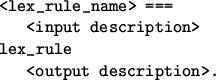
The format of lexical rule specifications for the lexical rule compiler is shown in figure 7.1. Note that this syntax is different from the lexical rule syntax of ALE , which also is provided by the TRALE system. As described in the ALE manual, lexical rules specified using the ALE lexical rule syntax result in expanding out the lexicon at compile time.

Figure 7.1: Lexical rule input syntax

A lexical rule consists of a lexical rule name, followed by the infix operator ===, followed by an input feature description, followed by the infix operator lex_rule, followed by an output feature description and ending with a period.

Input and output feature descriptions are ordinary descriptions as defined in the TRALE manual. The lexical compiler currently handles all kinds of descriptions except for path inequalities. Path equalities can be specified within the input or output descriptions, and also between the input and output descriptions.

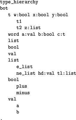
We illustrate the syntax with the small example grammar from Meurers and Minnen (1997), which is also included with the TRALE system in the subdirectory lr_compiler/examples. The signature of this example is shown in figure 7.2; to illustrate this TRALE signature syntax, figure 7.3 shows the type hierarchy in the common graphical notation.

Figure 7.2: An example signature

Figure 7.3: A graphical representation of the example type hierarchy

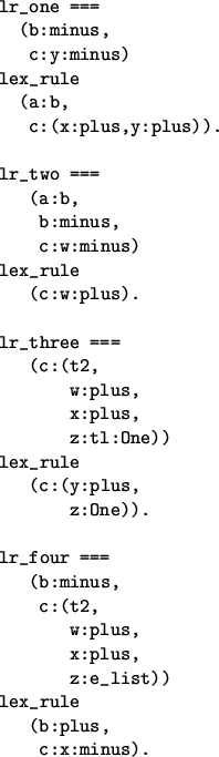
Based on this signature, figure 7.4 shows a set of four lexical rules exemplifying the lexical rule syntax used as input to the lexical rule compiler.

Figure 7.4: An example set of four lexical rule

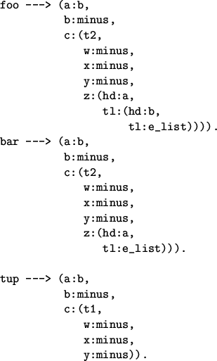
To complete the example grammar, we include three examples for base lexical entries in figure 7.5. These lexical entries can be found in the file lexicon.pl.

Figure 7.5: An example set of base lexical entries

The user is encouraged to look at this grammar, run the compiler on it, and make sure that the resulting output is consistent with the user's understanding. Visualizing the lexical rule interaction generally is a good way to check whether the intended lexical rule applications do in fact result from by the lexical rules that were specified in the grammar. The visualization obtained by calling lr_show_global/0 for the example grammar is shown in figure 7.6.

Figure 7.6: Global interaction visualization for the example grammar

The lexical rule interaction which is permitted by a particular lexical class can also be visualized. To view the automaton of an entry with the phonology Phon one calls lr_show_automaton(Phon). To view all such automata, the predicate to call is lr_show_automata/0. In figure 7.7 we see the visualization obtained for the lexical entry ``foo'' of our example grammar by calling show_automaton(foo).

Figure 7.7: Interaction visualization for the entry ``foo''

TRALE-EXTENSION:Interpretation

While the basic interpretation of lexical rules is straightforward, it turns out to be more difficult to answer the question how exactly the intuition should be spelled out that properties which are not changed by the output of a lexical rule are carried over unchanged, the so-called framing. A detailed discussion of the interpretation of lexical rules and the motivation for this particular interpretation can be found in Meurers (2001); we focus here on the essential ideas needed to sensibly use the lexical rule compiler.

A lexical rule can apply to a variety of lexical entities. While each of these lexical entities must be described by the input of the lexical rule in order for the rule to apply, other properties not specified by the lexical rule can and will vary between lexical entries. Feature structures corresponding to lexical entities undergoing the lexical rule therefore may differ in terms of type value and appropriate features. Frames carrying over properties not changed by the lexical rule need to take into account different feature geometries. Since framing utilizes structure sharing between input and output, we only need to be concerned with the different kinds of objects that can undergo a lexical rule with regard to the paths and subpaths mentioned in the output description. Specifically, when the objects undergoing lexical rule application differ with regard to type value along some path mentioned in the output description, we may need to take into account additional appropriate attributes in framing. Each such possibility will demand its own frame.

The lexical rule compiler provides a truthful procedural realization of the formal interpretation of lexical rules defined in Meurers (2001). Generally speaking, the input description of a lexical rule specifies enough information to capture the class of lexical entries intended by the user to serve as inputs. The output description, on the other hand, specifies what should change in the derivation. All other specifications of the input are supposed to stay the same in the output.

In the spirit of preserving as much information as possible from input to output, we generate frames on the basis of species (= most specific type) pairs; that is, we generate a frame (an IN-OUT pair) on the basis of a maximally specific input type, and a maximally specific output type, subtypes of those specified in, or inferred from, the lexical rule description. In this way we maintain tight control over which derivations we license, and we guarantee that all possible information is transferred, since the appropriate feature list we use is that of a maximally specific type. We create a pair of skeleton feature structures for the species pair, and it is to this pair of feature structures that we add path equalities. We determine the appropriate list of species pairs on the basis of the types of the input and output descriptions.

The first step in this process is determining the types of the input and output of the lexical rule. We then obtain the list of species of the input type, and the list of species of the output type. We refer to these as the input species list, and the output species list, and their members as input and output species. At this point it will be helpful to have an example to work with. Consider the type hierarchy in figure 7.8.

Figure 7.8: An example hierarchy for illustrating the interpretation

We can couch the relationship between the input and output types in terms of type unification, or in terms of species set relations. In terms of unification, there are four possibilities: the result of unification may be the input type, the output type, something else, or unification may fail. In the first case the input type is at least as or more specific, and the input species species will be a subset of the output species. In the second case the output is more specific and the output species will be a subset of the input species. In the third case the input and output types have a common subtype, and the intersection of input and output species is nonempty. In the fourth case the input and output types are incompatible, and the intersection of their species sets is empty.

If a (maximally specific) type value can be maintained in the output, it is. Otherwise, we map that input species to all output species. In terms of set membership, given a set of input species $X$, a set of output species $Y$, the set of species pairs $P$ thus can be defined as:

$$P = \begin{array}[t]{@{}l@{}} \{\langle x,x\rangle \mid x \i... ...angle \mid x \in X, x \not\in Y \wedge y \in Y\}\\ \end{array}$$

Given in figure 7.9

Figure 7.9: Examples for the four cases of mappings

are examples of all four cases, using the example signature, showing input and output types, the result of unification, their species lists, and the species-pairs licensed by the algorithm described below. Calling these separate ``cases'' is misleading, however, since the algorithm for deciding which mappings are licensed is the same in every case.